Hello guys, welcome back to my blog. Here in this article, I will discuss fixed-step solver in MATLAB Simulink, the types of fixed-step solver and which type of fixed step solver need to be selected.

Ask questions if you have any electrical, electronics, or computer science doubts. You can also catch me on Instagram – CS Electrical & Electronics

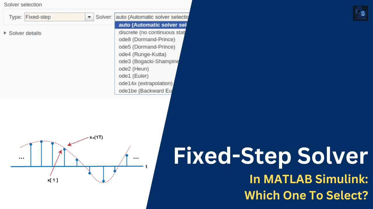
Fixed-Step Solver In MATLAB Simulink

Simulink, a simulation and model-based design tool from MATLAB, relies on numerical solvers to compute the system dynamics over time. These solvers are crucial for accurately simulating physical systems, control systems, and real-time applications.

Solvers in Simulink are broadly classified into fixed-step and variable-step solvers. Fixed-step solvers compute the system states at uniform time intervals, making them highly suitable for real-time applications, control systems, and embedded simulations where consistent execution timing is required.

Characteristics of Fixed-Step Solvers

Fixed-step solvers ensure deterministic execution, making them ideal for real-time systems where timing precision is crucial. These solvers maintain a constant step size throughout the simulation, which simplifies computation and improves predictability. However, they may suffer from lower accuracy when dealing with complex or highly dynamic systems due to their inability to adjust the step size dynamically.

Fixed-step solvers are generally preferred in applications such as digital control systems, power electronics, and hardware-in-the-loop (HIL) testing, where consistent time steps are necessary for synchronization with physical hardware.

Types of Fixed-Step Solvers in MATLAB Simulink and Their Applications

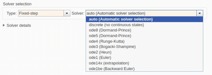
01. Auto Solver

The auto solver allows Simulink to automatically select the best fixed-step solver based on the system dynamics. This option is useful when the user is unsure about the most suitable solver for their specific application.

Applications: General-purpose simulation models, initial solver selection for embedded applications.

02. Discrete Solver

The discrete solver is designed for purely discrete models, meaning there are no continuous states involved. It is commonly used in digital control systems, event-driven models, and systems that utilize zero-order hold (ZOH) and first-order hold (FOH) discretization techniques.

Applications: Digital control systems, logic-based control, sampled-data systems.

03. ODE1 (Euler’s Method)

ODE1 is the simplest numerical integration method among fixed-step solvers. It follows a basic forward Euler approach and is computationally efficient. However, it has low accuracy and is less stable, making it suitable only for simple models or real-time applications where computational efficiency is prioritized over precision.

Applications: Basic real-time simulations, fast-executing models, simple embedded controllers.

04. ODE2 (Heun’s Method)

ODE2, also known as Heun’s method, provides better accuracy than ODE1 by taking an intermediate step before updating the system state. It is commonly used in digital control applications where moderate accuracy is required while maintaining computational efficiency.

Applications: Control system modeling, robotics control, digital controllers.

05. ODE3 (Bogacki–Shampine Method)

ODE3 is a third-order Runge-Kutta method, offering improved accuracy compared to ODE1 and ODE2. It is particularly useful in moderate-accuracy real-time applications where computational efficiency and accuracy must be balanced.

Applications: Sensor fusion algorithms, predictive control, adaptive control systems.

06. ODE4 (Classical Runge-Kutta Method)

ODE4 is widely used in numerical simulations due to its high accuracy. It is a fourth-order Runge-Kutta method that provides a good balance between computational efficiency and precision. ODE4 is suitable for most control system simulations that require reliable accuracy without excessive computational load.

Applications: Aerospace and automotive control systems, PID tuning, power electronics modeling.

07. ODE5 (Dormand-Prince Method)

ODE5 is a fifth-order Runge-Kutta method that enhances accuracy compared to ODE4. It is used in control and signal processing applications where higher precision is necessary. This solver is effective in applications requiring more accurate state estimations while maintaining reasonable computational efficiency.

Applications: High-precision motion control, DSP applications, real-time embedded control.

08. ODE8 (Fehlberg Method)

ODE8 is an eighth-order Runge-Kutta method, providing extremely high accuracy. It is mainly used in simulations where precision is critical, such as high-precision modeling of dynamic systems.

Applications: Spacecraft trajectory simulation, high-fidelity vehicle dynamics, advanced control systems.

09. ODE14x (Extrapolation Method)

ODE14x is specifically designed for handling stiff systems. It employs extrapolation techniques to improve accuracy and stability in simulations where rapid changes in dynamics occur. This solver is particularly useful in power electronics, stiff ODE problems, and circuit simulations.

Applications: Power electronics circuits, chemical process modeling, electric grid stability analysis.

10. ODE1be (Backward Euler Method)

ODE1be is an implicit solver used for stiff systems. Unlike explicit methods, it evaluates system states by solving an implicit equation at each step, making it more stable for highly stiff models. It is widely applied in power electronics, stiff ODEs, and scenarios where numerical stability is a concern.

Applications: Power grid stability, stiff mechanical system simulations, thermal modeling.

Comparison of Fixed-Step Solvers

Solver	Order	Accuracy	Computational Cost	Stability
ODE1	1	Low	Low	Low
ODE2	2	Medium	Low	Medium
ODE3	3	Medium	Medium	Medium
ODE4	4	High	Medium	High
ODE5	5	High	Medium-High	High
ODE8	8	Very High	High	Very High
ODE14x	–	High	High	Very High
ODE1be	1 (Implicit)	Medium	High	Very High

Common Challenges and Mitigation Strategies

Numerical Instability

Challenge: Some solvers become unstable when used with large step sizes.
Mitigation: Use solvers like ODE1be or ODE14x for stiff systems, and reduce the step size if necessary.

Computational Load

Challenge: High-order solvers require more processing power.
Mitigation: Use lower-order solvers like ODE1 or ODE2 when computational efficiency is a priority.

Step Size Selection

Challenge: A large step size reduces accuracy, while a small step size increases computation time.
Mitigation: Optimize step size based on system dynamics and simulation requirements.

Real-Time Constraints

Challenge: Some solvers may not meet real-time execution requirements.
Mitigation: Choose efficient solvers like ODE1 or ODE2 for real-time systems with limited resources.

Conclusion

Fixed-step solvers play a crucial role in real-time and embedded system simulations. They provide deterministic execution timing and simplify numerical integration while requiring careful selection based on accuracy and system dynamics. By understanding the strengths and limitations of different fixed-step solvers, engineers can optimize simulations for control systems, power electronics, and various real-time applications.

This was about “Fixed-Step Solver In MATLAB Simulink“. Thank you for reading.

Also, read:

About The Author

Chetan Shidling

Automotive | Technical Blogger | Engineer | Content Creator

See author's posts

Share Now