What Is Time Complexity, Calculation, Examples, Types

November 3, 2022November 3, 2022 CS Electrical And Electronics

Hello guys, Welcome back to our blog. Here in this article, we will discuss what is time complexity, how time complexity is calculated, examples, and what are the different types of time complexity.

If you have any electrical, electronics, and computer science doubts, then ask questions. You can also catch me on Instagram – CS Electrical & Electronics.

Also, read the following:

What Is Time Complexity

The Time Complexity of a program is the amount of time the program takes to run, as a function of the length of the input. It measures the time taken to execute each statement of code in a program. It gives information about the variation in the execution time of the program.

The time_complexity of a program is not the exact time needed to execute a certain code, since that depends on different factors like a programming language, operating software, processing power, etc. The idea behind time_complexity is that it can measure solely the execution time of the program in a way that depends only on the program itself and its input.

Significance of Time Complexity:

The Time Complexity of a program is significant as it quantifies the amount of time taken by a program to run as a function of the length of the input.

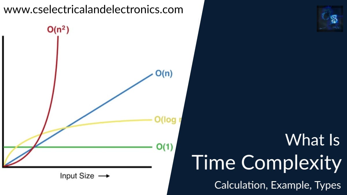
The “Big O notation expresses the time_complexity of a program”. The Big O notation is a language that simply states the existing relationship between the input data size (n) and the number of operations performed (N) with respect to time.

Big O notation represents the run time of a program in terms of how fast it grows relative to the input (this input is called “n”). This way, if the run time of an algorithm grows “on the order of the size of the input”, it would be stated as “O(n)”. If the run time of an algorithm grows “on the order of the square of the size of the input”, it would express it as “O(n²)”.

This relation is designated as the order of growth in time_complexity and is given the notation “O[n]” where O is the order of growth and n is the length of the input.

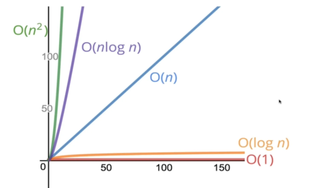
There are different types of time complexities:

01. Constant time – O(1)

Programs with Constant Time-Complexity take a constant amount of time to run, independent of the size of the input. These programs are the fastest programs as they do not alter their run-time in response to the size of the input data.

Example of Constant Time Complexity is :

[ name = “Your Name”
            print(name)               ]

The above-given example will run in one step, so its complexity will be O(1).

02. Linear Time Complexity – O(n)

When the Time Complexity is directly proportional to the size of the input (n) then the program is said to have a Linear Time_Complexity.

Programs with linear time_complexity will process the input(n) in the “n” number of operations. And so, this means that the time taken by the program to complete will be directly proportional to the size of the input.

Example of Linear Time Complexity :

[  def print_names (name list) :
         for name in name_list :
              print (name)                 ]

The above example will run n times, thus, its Time Complexity will be O(n).

Here the number n depends on the number of names in the list.

03. Logarithmic Time Complexity – O(log n)

A program is said to be in Logarithm Time_Complexity when the size of input data is reduced with each step, this is achieved by making the time execution proportional to the logarithm of the input size.

What this means is that the time taken by the program to complete is inversely proportional to the size of the input(n). This makes the Logarithmic Time Complexity faster than Linear Time_Complexity, but not faster than Constant Time_Complexity.

Example of Logarithmic Time Complexity :

[  def power_of_2(a) :
         x = 0
               while a>1:
                     a = a//2 
                     x = x+1

   return x                    ]

04. Quadratic Time Complexity: O(n^2)

In a Quadratic Time Complexity program, the time taken to complete the program is directly proportional to the square of the size of the input data (n^2).

Normally, nested loops run under quadratic time complexity, as a linear operation is run within another linear operation(n*n).

In programs with large data sets, Quadratic Time Complexity takes a longer time to complete and a lot of resources and time are required, thus the user is better off with other time complexities.

Example of Quadratic Time Complexity:

[ def print_first_last_name(name_list) :
        for names in name_list :
             For name in names :
                    print(name)

Name_list = [ {“Name1”, “Name2”, “Name3”, …, “NameN”}, {“SName1”, “SName2”, “SName3”, …., “SNameN”} ]

In the above example, a nested loop has been used, so that the program will run for n number of times for the first loop then n number of times for the second loop, and then the time_complexity will be n*n= n^2.

How to measure time complexity:

Idea 1: The easiest way to measure the execution time of a program across platforms is to count the measure of steps.

Idea 2: Then the number of steps can be represented with algebra.

Idea 3: The most critical part of the representation is the greatest power if n. For example, consider 3n+5. As n increases in value, the 5 part becomes less and less important. And, in the case of n^2+n, the alone n becomes less important.

The Big O notation is the logical continuation of the above three ideas. The number of steps is converted to a formula, and then only the highest power of n is used to represent the entire program.

Time Complexity of Sorting Algorithm

The Sorting Algorithm arranges and rearranges sets of data elements of an array so that they can be placed either in ascending or descending order.

01. Time Complexity of Insertion sort

Insertion sort is one of the intuitive sorting programs for beginners which shares an analogy with the way a person sorts the cards dealt in their hands. This algorithm is based on the assumption that a single element is always sorted.

How it works

Compare the element with its adjacent element.
If at every comparison, we could find a position in the sorted array where the element can be inserted, then the space is created by shifting the elements to the right and then the element is inserted in the appropriate position.
Then the above steps are repeated until the last element of the unsorted array to its correct position.

Works Case Time_Complexity of Insertion Sort – O(n^2)

Best Case Time Complexity of Insertion Sort – O(n)

02. Time Complexity of Merge Sort

Merge sort is a sorting algorithm in which it splits the input into similar parts until solely two numbers are there for comparison and then after comparing and covering each part it merges them all together back to the input.

How it works

The first step is to divide the input into two halves which comprises the use of logarithmic time complexity. i.e, log(n) where n is the number of elements.
The second step is to merge back the array into a single array, so if we observe it in all number of elements to be merged n, and to merge back we use a single loop that runs over all the N elements giving it Time_Complexity of O(n).
Finally, the total time complexity will be STEP1 + STEP2.

Best Case of Time Complexity of Merge Sort – O(n long)

03. Time Complexity of Bubble Sort

Bubble sorting is one of the most straightforward brute-force sorting algorithms. It is utilized to sort elements in either ascending or descending hierarchy by comparing each and every element with the other in bubble sort. A nested loop is used to execute this program.

The best case of Time Complexity of Bubble Sort – O(n)

The worst case of Time_Complexity of Bubble Sort – O(n^2)

04. Time Complexity of Quick Sort

The Quick Sort is a sorting algorithm that uses the divide and conquers method.

In quick sort, an element is chosen as the pivot and a partition of an array is created around that pivot. By repeating this technique for each partition the arrays get sorted

depending on the position of the pivot.

Quick Sort can be applied in different ways:

taking the first or last element as a pivot
taking the median element as a pivot

Time Complexity of Searching Algorithm

A search algorithm is designed to check for an element or retrieve an element from any data structure where it is stored or to locate specified data in the collection of data.

01. Time Complexity of Linear Search:

Linear search (known as sequential search) is an algorithm for finding a target value within a list. It sequentially checks each element of the list for the target value until a match is found or until all the elements have been searched.

How it works

The first element is selected as the current element
The current element is compared with the target element. If the target element matches with the current element then the location of the target element(which is the location of the current element which was searched against the target element) is returned.
If the first element did not match the target element then the next element is selected as the target element and is searched against the target element in the data size. If the current element matches the target element the location is returned. Else, the next element is taken as the current element and is searched against the data.
This process continues until the current element matches the target element.

The best case will take place if the element to be searched is on the first index. The number of comparisons in this place will be 1. Therefore, the Best Case of Time_Complexity of Linear Search will be O(1).

The worst case will take place if the element to be searched is in the last index or if the element to be searched is not present in the list. In both cases, the maximum number of comparisons that take place in linear search will be equal to n number of comparisons. Thus, the worst case of time complexity of linear search will be O(n).

02. Time Complexity of Binary Search

Binary Search is the algorithm that efficiently searches an element in a given list of sorted elements. Binary Search lessens the size of the data fixed to search by half at each step.

Binary Search is the faster of the two searching algorithms. However, with smaller arrays, linear search does a better job.

The best case of binary search is when the element to be searched is in the middle of the list. As the element is in the middle of the list and can be found in the first round of search thus there is only 1 comparison which makes the Time_Complexity of Binary Search O(1).

The worst case of time complexity of the binary search is when the element to be searched is found in the first or last index. As the element is in the first or last index the total number of comparisons required is logN comparisons which make the Time_Complexity of Binary Search O(long).

This was about “What Is Time Complexity“. I hope this article may help you all a lot. Thank you for reading.

Also, read: