Hello guys, welcome back to our blog. In this article, I will discuss variable-step solvers in MATLAB Simulink, the types of variable-step solvers, and which types of variable-step solvers need to be selected.

Ask questions if you have any electrical, electronics, or computer science doubts. You can also catch me on Instagram – CS Electrical & Electronics

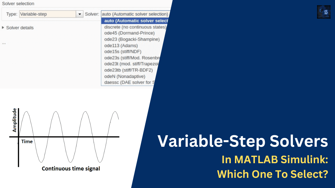
Variable-Step Solvers In MATLAB Simulink

Variable-step solvers in MATLAB Simulink play a crucial role in accurately modeling and simulating dynamic systems. Unlike fixed-step solvers, which use a constant step size, variable-step solvers adapt the step size dynamically based on system behavior. This flexibility improves efficiency by taking larger steps when system changes are gradual and smaller steps when system changes are rapid.

Variable-step solvers are widely used in applications that require high accuracy, efficient computational performance, and adaptive step-size control, such as aerospace systems, automotive simulations, power electronics, and control systems. These solvers help in managing stiff and non-stiff systems, providing optimal trade-offs between accuracy and performance.

Characteristics of Variable-Step Solvers

Adaptive Step Size: Adjusts step size based on error tolerance and system dynamics.
Efficiency: Reduces computational cost by minimizing unnecessary computations in smooth regions.
Accuracy: It provides higher precision compared to fixed-step solvers, especially in rapidly changing systems.
Suitability for Stiff Systems: Some solvers handle stiff systems more effectively by employing implicit numerical methods.

Types of Variable-Step Solvers in MATLAB Simulink and Their Applications

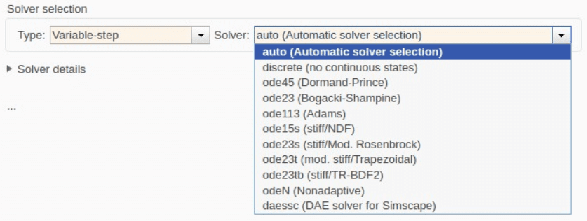
01. Auto Solver

The auto solver automatically selects the best variable-step solver based on system dynamics. It evaluates the model and assigns the most appropriate solver for efficiency and accuracy.

Applications: General-purpose modeling, initial solver selection, adaptive simulations.

02. Discrete Solver

The discrete solver is used for systems with discrete states and event-driven models. It does not solve continuous differential equations but is useful in hybrid discrete-continuous simulations.

Applications: Digital control systems, event-driven systems, logic-based simulations.

03. ODE45 (Dormand-Prince Method)

ODE45 is a fourth- and fifth-order Runge-Kutta solver. It is widely used for non-stiff problems where moderate accuracy and efficiency are required. It balances computational cost and precision effectively.

Applications: Control systems, mechanical simulations, trajectory analysis, robotics.

04. ODE23 (Bogacki-Shampine Method)

ODE23 is a third-order Runge-Kutta method with an adaptive step-size control. It is faster but less accurate than ODE45 and is ideal for problems requiring quick execution with reasonable accuracy.

Applications: Real-time systems, signal processing, approximate control applications.

05. ODE113 (Variable-Order Adams-Bashforth-Moulton Method)

ODE113 uses a variable-order, multi-step Adams-Bashforth-Moulton method. It is more efficient for problems where high precision is needed without excessive computational overhead.

Applications: Long-term orbital simulations, precise electrical circuit modeling.

06. ODE15s (Backward Differentiation Formula – BDF)

ODE15s is designed for stiff differential equations and employs implicit numerical integration methods. It is more stable for highly dynamic and stiff problems where explicit solvers fail.

Applications: Chemical reactions, power systems, thermal systems, biomedical modeling.

07. ODE23s (Modified Rosenbrock Method)

ODE23s is a second-order solver specifically designed for stiff systems. It is computationally efficient and works well for problems where high accuracy is not the primary concern.

Applications: Power converters, electrical grids, constrained mechanical systems.

08. ODE23t (Trapezoidal Rule)

ODE23t is an implicit solver based on the trapezoidal rule, suitable for mildly stiff problems. It balances efficiency and stability while maintaining reasonable accuracy.

Applications: Hydraulic systems, fluid dynamics, thermal management.

09. ODE23tb (Trapezoidal Rule with Backward Differentiation Formula)

ODE23tb extends the trapezoidal method by incorporating a backward differentiation approach for improved stability in stiff problems. It is useful when other solvers struggle with numerical stability.

Applications: Power electronics, network simulations, and semiconductor modeling.

10. ODEN (Custom User-Defined Solvers)

ODEN allows users to implement their own solver algorithms, providing flexibility to tailor numerical integration to specific system needs.

Applications: Custom engineering solutions, research applications, experimental control systems.

11. daessc (Differential-Algebraic Equation Solver)

daessc is specifically designed for differential-algebraic systems, where some equations contain algebraic constraints. It ensures consistency in solving such complex problems.

Applications: Mechanical linkages, electrical circuit simulations, constrained dynamic systems.

Comparison of Variable-Step Solvers

Solver	Order	Accuracy	Computational Cost	Stability	Suitable for Stiff Problems
ODE45	4/5	High	Medium	Medium	No
ODE23	2/3	Medium	Low	Medium	No
ODE113	Variable	High	Medium	High	No
ODE15s	Variable	High	Medium-High	Very High	Yes
ODE23s	2	Medium	Low	High	Yes
ODE23t	2	Medium	Medium	Medium	Yes
ODE23tb	2	Medium-High	Medium	High	Yes
daessc	Variable	High	High	High	Yes

Common Challenges and Mitigation Strategies

01. Numerical Instability

Challenge: Some solvers become unstable for stiff problems.
Mitigation: Use stiff solvers like ODE15s, ODE23s, or ODE23tb.

02. High Computational Cost

Challenge: High-order solvers require more processing power.
Mitigation: Use lower-order solvers like ODE23 for real-time applications.

03. Step Size Selection

Challenge: A large step size reduces accuracy, while a small step size increases computational load.
Mitigation: Optimize solver tolerances and initial conditions for better performance.

04. Stiff Systems Handling

Challenge: Non-stiff solvers struggle with stiff problems.
Mitigation: Use implicit solvers such as ODE15s and ODE23s for better stability.

Conclusion

Variable-step solvers in MATLAB Simulink provide powerful capabilities for accurately modeling and simulating dynamic systems. By dynamically adjusting step sizes, they enhance computational efficiency and precision. Selecting the right solver depends on system characteristics, accuracy requirements, and computational constraints. Understanding the differences and applications of each solver ensures optimal performance in engineering simulations across various industries, including automotive, aerospace, power electronics, and robotics.

This was about “Variable-Step Solvers In MATLAB Simulink“. Thank you for reading.

Also, read:

About The Author

Chetan Shidling

Automotive | Technical Blogger | Engineer | Content Creator

See author's posts

Share Now